UMAP dimension reduction

UMAP: Uniform Manifold Approximation and Projection for Dimension Reduction.

UMAP is a novel manifold learning technique for dimension reduction. UMAP is constructed from a theoretical framework based in Riemannian geometry and algebraic topology. The result is a practical scalable algorithm that applies to real world data. The UMAP algorithm is competitive with t-SNE for visualization quality, and arguably preserves more of the global structure with superior run time performance. Furthermore, UMAP has no computational restrictions on embedding dimension, making it viable as a general purpose dimension reduction technique for machine learning.

Spectra selection, normalization and previsualization

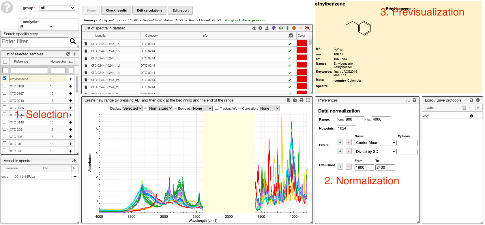
The first step is to select the spectra :

Select spectra

How to select spectra.

Spectra selection

All the spectra analysis tools start with a phase of selection.

Select samples

In order to facilitate the analysis of the spectra it is advised to have samples containing representative spectra in order to evaluate the intra-variability as well as the reproducibility.

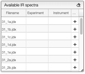
Selection of spectra to analyze is achieved with one of those 3 methods:

At the level of the sample by either clicking on the +, this will add all the spectra related to this sample or on the + on the top of the sample box to add all the spectra of all the selected samples.

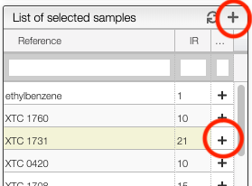
If you select a sample it is also possible to add a specific spectrum by clicking on the + at the level of the spectra list.

Once spectra have been selected, data normalization filters can be applied :

Spectrum preprocessing

Apply mathematical tools to the spectra.

Preprocessing

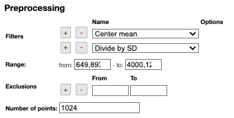
Filters

You can apply the following filters to the spectra to enhance the visualization. The modifications include the following:

• Center Mean : subtract the mean from every variable observation in the dataset, so that the new variable's mean is centered at 0.
• Center Median : subtract the median from every variable observation in the dataset, so that the new variable's median is centered at 0`
• Divide by SD : divide every variable observable in the dataset by the standard deviation yields a distribution with a standard deviation equal to 1.
• Normed: Specify a value in the value field and select the type of normalization:
  • Sum to value: normalize the integral under the curve so that it sums to the specified value.
  • Absolute sum to value: normalize the integral under the curve so that the absolute sum sums to the specified value.
  • Max to value: normalize the maximum value to the specified value.
• Rescale (x to y) : rescale the graph such that the y-values fit between specified minimum and maximum values.
• First derivative : calculate the first derivative of the spectra.
• Second derivative : calculate the second derivative of the spectra.
• Third derivative : calculate the third derivative of the spectra.
• Savitzky-Golay : smooth the spectra and calculate derivatives based on the following parameters:
  • Window: smoothing window size, must be an odd number, greater than 5.
  • Derivative: derivative order.
  • Polynomial: the degree of the polynomial used to calculate the Savitzky-Golay.
• AirPLS baseline : baseline correction using adaptive iterative reweighed penalized least squares algorithm.
• Iterative polynomial baseline : baseline correction using iterative polynomial fitting algorithm.
• Rolling average baseline : baseline correction using a rolling average.
• Rolling median baseline : baseline correction using a rolling median.
• Rolling ball baseline : baseline correction using a rolling ball.
• Ensure growing X values: ensure that the x-values are in increasing order.
• Function on X : apply a function to the x-values. For example, log(x).
• Function on Y : apply a function to the y-values. For example, log10(y+1).
• Calibrate X : calibrate the x-values with the parameters from, to, nbPeak and targetX.
• Pareto normalization : Pareto scaling, which uses the square root of standard deviation as the scaling factor, circumvents the amplification of noise by retaining a small portion of magnitude information. 10.1016/j.molstruc.2007.12.026

One classical preprocessing algorithm is Standard Normal Variate (SNV). This preprocessing can be achieved by selecting the 2 options Center mean and Divide by SD.

Selecting the range

A certain range of x-values can be selected to show only a part of the spectrum using Range.

Exclusions

Depending on the analysis, some regions should be removed using Exclusions in order to improve the visualization.

Number of points

Number of points can be changed to reduce the number of points in the spectra.

The superimposed spectra can be manipulated without numerous :

Visualization

How to visualize spectra.

Spectra visualization

Numerous options are available to display the either all the spectra in the dataset or the selected spectra in the dataset.

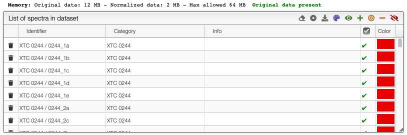
Selection of spectra in the dataset

The toolbar on the top of the list of spectra in the dataset provides many options (from left to right):

• Remove all spectra from dataset
• Select category: select which property contains the category description
• Download normalized matrix
• Recolor spectra based on category: a different color will be applied for each category. By default, the sample reference
• Select all spectra
• Append to selected spectra
• Select only current spectra
• Remove spectra from current selection
• Unselect all spectra

Graph options

It is possible to either display the selected spectra, all the spectra or various derived information.

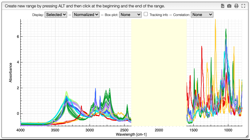
Customization of the display is achieved using the chart toolbar:

Display spectra

The first options allow to either display all the spectra, only the selected spectra or nothing.

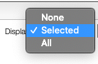
Displaying no spectrum is useful when displaying other derived data.

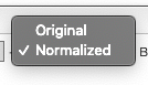
Original / normalized

These options allow to either display the original spectra or the normalized data. Most of the time we will display normalized data. Those are the data that will be analyzed, and normally they also take less room in memory.

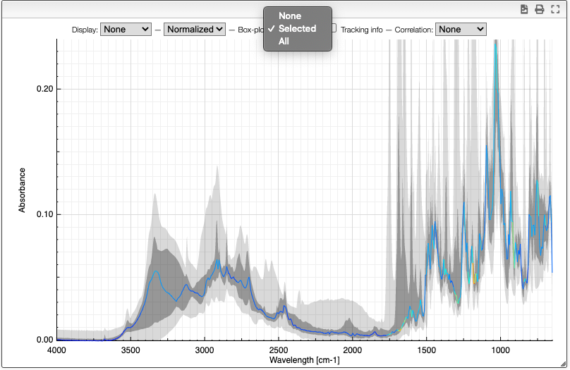
Boxplot

The boxplot kind of representation allows to display the first / third quartile as a dark grey zone for each X point. The min and max values are represented as a light gray zone and the median is represented as a line for which the color varies based on the standard deviation (red: high variation, blue: small variation).

Tracking information

By selecting the tracking information you will display the X values and the corresponding Y values for all the spectra.

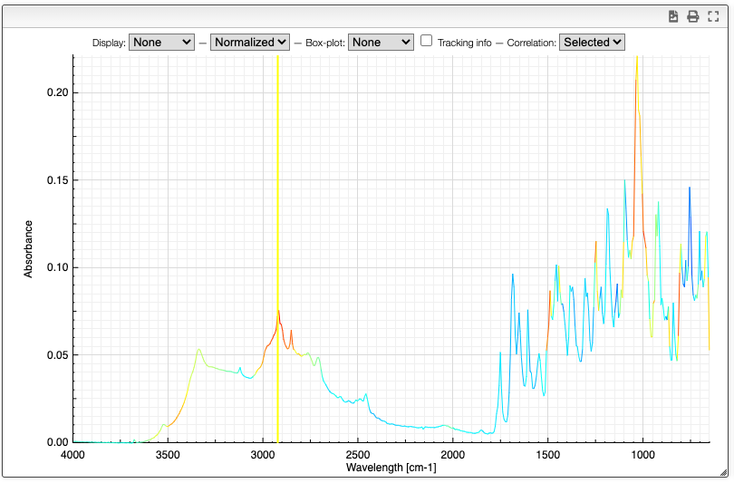
Correlation

Correlation of the vector represented by the Y points can be useful to determine which peaks are correlated in a big mixture of products. This is known in NMR metabolomics as STOCSY.

By SHIFT ⇧ + ALT + click you can select the X value for which you would like to check correlation. Strongly correlated signals will appear in red while non correlated signals are blue.

References

• https://arxiv.org/abs/1802.03426