Permeability

Theoretical background

Permeability is a phenomenon where molecules diffuse through a solid. This phenomenon can be modeled by Fick's law of diffusion.

Fick's law of diffusion

The flux (or flow of mass) is proportional to the gradient of the concentration. In one dimension, Fick's first law of diffusion if given by,

$$J = -D \frac{\partial \phi}{\partial x}$$

Where $J$ is the flux, $D$ is the mass diffusivity, and $\phi$ is the concentration of gas. The above equation can be approximated by the relation

$$J = -D \frac{(C_2 - C_1)}{\delta}$$

Where $C$ is the concentration at the edge and $\delta$ is the thickness of the membrane.

Upload spectrum

You can upload a spectrum either as JCAMP or TXT format.

Spectra analysis

In the graph view, it is possible to superimpose multiple y variables, in order to have a more global view of the different variables.

Plot multiple y variables

You can superimpose multiple curve on the same plot.

This tool allows you to visualize multiple entries on the same graph. For example, the permeability of methane, nitrogen, and oxygen can be visualized simultaneously. You can select, in the y axis menu, the variables that you want to see.

Every curve will be plotted with a different color, and you can zoom in by selecting the area you want and zoom out by double-clicking on the graph. Additionally, you can hide and show curves by clicking on the corresponding eye at the bottom of the graph.

You can also apply mathematical processing to the curves via the preprocessing panel.

Spectrum preprocessing

Apply mathematical tools to the spectra.

Preprocessing

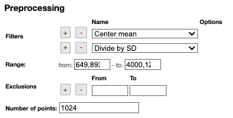
Filters

You can apply the following filters to the spectra to enhance the visualization. The modifications include the following:

• Center Mean : subtract the mean from every variable observation in the dataset, so that the new variable's mean is centered at 0.
• Center Median : subtract the median from every variable observation in the dataset, so that the new variable's median is centered at 0`
• Divide by SD : divide every variable observable in the dataset by the standard deviation yields a distribution with a standard deviation equal to 1.
• Normed: Specify a value in the value field and select the type of normalization:
  • Sum to value: normalize the integral under the curve so that it sums to the specified value.
  • Absolute sum to value: normalize the integral under the curve so that the absolute sum sums to the specified value.
  • Max to value: normalize the maximum value to the specified value.
• Rescale (x to y) : rescale the graph such that the y-values fit between specified minimum and maximum values.
• First derivative : calculate the first derivative of the spectra.
• Second derivative : calculate the second derivative of the spectra.
• Third derivative : calculate the third derivative of the spectra.
• Savitzky-Golay : smooth the spectra and calculate derivatives based on the following parameters:
  • Window: smoothing window size, must be an odd number, greater than 5.
  • Derivative: derivative order.
  • Polynomial: the degree of the polynomial used to calculate the Savitzky-Golay.
• AirPLS baseline : baseline correction using adaptive iterative reweighed penalized least squares algorithm.
• Iterative polynomial baseline : baseline correction using iterative polynomial fitting algorithm.
• Rolling average baseline : baseline correction using a rolling average.
• Rolling median baseline : baseline correction using a rolling median.
• Rolling ball baseline : baseline correction using a rolling ball.
• Ensure growing X values: ensure that the x-values are in increasing order.
• Function on X : apply a function to the x-values. For example, log(x).
• Function on Y : apply a function to the y-values. For example, log10(y+1).
• Calibrate X : calibrate the x-values with the parameters from, to, nbPeak and targetX.
• Pareto normalization : Pareto scaling, which uses the square root of standard deviation as the scaling factor, circumvents the amplification of noise by retaining a small portion of magnitude information. 10.1016/j.molstruc.2007.12.026

One classical preprocessing algorithm is Standard Normal Variate (SNV). This preprocessing can be achieved by selecting the 2 options Center mean and Divide by SD.

Selecting the range

A certain range of x-values can be selected to show only a part of the spectrum using Range.

Exclusions

Depending on the analysis, some regions should be removed using Exclusions in order to improve the visualization.

Number of points

Number of points can be changed to reduce the number of points in the spectra.

Columns customization

In many tables it is possible to select which columns to display. This is achieved by clicking on the icon.

After clicking on the icon a dialog box opens that allows to add a new column.

There are 5 parameters to fill for a new column:

• name: the column name. This will be displayed as the header to the column.
• rendererOptions: options that allows among other to format numbers. One very useful formatter is numeral (see after)
• width: number of pixels for the specific column. May stay empty for automatic layout.
• forceType: select how to display complex values (see later)
• jpath: where to find the information to display in the column

In order to add a new column you need to select the jpath using the hierarchical drop down menu.

Columns can be moved or rearranged as well.

rendererOptions: numeral

number,

Value to format	rendererOptions	Result
12.345678	numeral:'#.##'	12.34
12.3	numeral:'#.00'	12.30
0.3	numeral:'#.0 %'	30.0 %

forceType

In the database some values are stored as an object that needs to be displayed to the user in an intuitive way.

For example the unit type will store in the database the value using as units SI (we convert the data to the units defined by the 'standard international') and specify in which units the user would like to display the data. So in the following example we are in fact storing the value -150°C by storing the value in SI (Kelvin) and specifying that the user wants to see it in °C.

{
  "SI": 123.15,
  "unit": "°C"
}

Another example is the valueUnits type that will store the data in 2 different properties (value and unit). In this case the value is stored in the specified units and there is no conversions.

{
  "value": 123,
  "units": "°C"
}

While this way to store the data in the database is very practical it is not the way that the user would like to see his results. We have therefore the possibility to forceType: define how the user would like to see the results.

Other types include mf. This formatter allows to correctly display a molecular formula that is stored in the database as "C10H20O3". i.e. it will put the numbers in subscript (C₁₀H₂₀O₃).

References

1. Permeability