Isotherm analysis

Introduction

Adsorption is a process of adhesion of atoms, ions or molecules on a surface. Desorption is the inverse process. There are two types of adsorption:

• Physisorption: Atoms and molecules are trapped on the surface of solid due to attractive Van der Waals forces.
• Chemisorption: Adsorption that involves a chemical reaction between the surface and the absorbate (example : corrosion).

These adsorptions can be described by adsorption isotherms. If the adsorbate is a gas, its amount is plotted against its pressure, if it consists of a liquid phase solute, it is plotted as a function of the concentration. In both cases, the process occurs at a constant temperature.

There are several models to describe adsorption. For example the Langmuir adsorption Isotherm or the BET Theory.

Langmuir Adsorption Isotherm

The following assumptions are made :

• The surface has finite number of identical adsorption sites $N$.
• There can be only a single adsorbate per site ($\theta_{\text{max}} = 1$: monolayer).
• The enthalpy of adsorption ($\Delta H_{\text{abs}}$) is independent of the coverage $\theta$, we suppose no interaction between the adsorbates.

If $K_a$ is the equilibrium constant and $p_a$ the partial pressure of the gas, the coverage is given by the Langmuir isotherm:

$$\theta = \frac{K_a p_a}{1+K_a p_a}, \quad \theta \in [0, 1]$$

Limitations of the Langmuir model

In this model, the interactions between the adsorbed molecules are neglected and it is only a monolayer adsorption.

BET (Brunauer–Emmett–Teller) Theory

This model allows multilayer adsorption. The following assumptions are made :

• Gas molecules physically adsorb on a solid in layers infinitely.
• Gas molecules only interact with adjacent layers.
• The Langmuir model can be applied to each layer.
• The enthalpy of adsorption for the first layer is constant and greater than the second (and higher).
• The enthalpy of adsorption for the second (and higher) layers is the same as the enthalpy of liquefaction.

With these assumptions, the BET equation is given as :

$$\theta=\frac{cp}{(1-p/p_o)\bigl(p_o+p(c-1)\bigr)}$$

Where $c$ is the BET $c$-constant, $p_o$ is the vapor pressure of the adsorptive bulk liquid phase and $\theta$ is the surface coverage.

Upload a file

Files can be uploaded either by drag-and-drop to the field on the left-hand-side or automatically from the instrument. The files will appear in field 2. Note that you can only upload files to samples to which you have write access.

Supported file types

We currently support the file types (which are also automatically detected):

• xls files produces by Belsorp instruments
• csv files produced by Belsorp instruments
• txt files produced by IGA instruments
• txt files produced by micrometrics instruments
• csv files produced by micrometrics instruments

If multiple desorption/adsorption cycles are stored in one file they will also be converted to one JCAMP file by our parsers.

If you need support for other file formats, open an issue on the GitHub repository or post a question in the user forum.

Visualization

This graph analysis use a dropdown menu switcher. If there are multiple experiments or columns in a file, you can select the ones that you want to plot using the dropdown selectors.

Dropdown menu for spectrum anaysis

It is possible to see the dependance of one variable as a function of another.

At the top of the graph, you can see three dropdown menus.

The first one is the choice of either all curve or either adsorption or desorption. The two other menus are the variables that you want to show as a dependence.

You can manipulate the graph in the same way than the IR spectrum graph.

At the top of the graph, you can export the image as a svg file, you can remove the grid or even export as a pdf file.

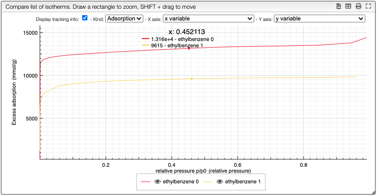
Compare data

By clicking on the button Compare, you can compare multiple isotherms. You can also select which curve you want to plot and choose the color.

Visualising spectra

How to show/hide spectra.

Visualising spectra

If you wish to see only certain spectra, it is possible to selectively hide (or delete) them.

In order to do so, use the buttons on the top panel of the displayed spectra list.

You can also change the color of an individual spectrum in the displayed spectra tab with a double click.

note

You can still still select the adsorption/desorption as well as the multivariable dependance.

The right box can be use to hide regions of the graph or take the derivative for example.

Spectrum preprocessing

Apply mathematical tools to the spectra.

Preprocessing

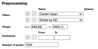
Filters

You can apply the following filters to the spectra to enhance the visualization. The modifications include the following:

• Center Mean : subtract the mean from every variable observation in the dataset, so that the new variable's mean is centered at 0.
• Center Median : subtract the median from every variable observation in the dataset, so that the new variable's median is centered at 0`
• Divide by SD : divide every variable observable in the dataset by the standard deviation yields a distribution with a standard deviation equal to 1.
• Normed: Specify a value in the value field and select the type of normalization:
  • Sum to value: normalize the integral under the curve so that it sums to the specified value.
  • Absolute sum to value: normalize the integral under the curve so that the absolute sum sums to the specified value.
  • Max to value: normalize the maximum value to the specified value.
• Rescale (x to y) : rescale the graph such that the y-values fit between specified minimum and maximum values.
• First derivative : calculate the first derivative of the spectra.
• Second derivative : calculate the second derivative of the spectra.
• Third derivative : calculate the third derivative of the spectra.
• Savitzky-Golay : smooth the spectra and calculate derivatives based on the following parameters:
  • Window: smoothing window size, must be an odd number, greater than 5.
  • Derivative: derivative order.
  • Polynomial: the degree of the polynomial used to calculate the Savitzky-Golay.
• AirPLS baseline : baseline correction using adaptive iterative reweighed penalized least squares algorithm.
• Iterative polynomial baseline : baseline correction using iterative polynomial fitting algorithm.
• Rolling average baseline : baseline correction using a rolling average.
• Rolling median baseline : baseline correction using a rolling median.
• Rolling ball baseline : baseline correction using a rolling ball.
• Ensure growing X values: ensure that the x-values are in increasing order.
• Function on X : apply a function to the x-values. For example, log(x).
• Function on Y : apply a function to the y-values. For example, log10(y+1).
• Calibrate X : calibrate the x-values with the parameters from, to, nbPeak and targetX.
• Pareto normalization : Pareto scaling, which uses the square root of standard deviation as the scaling factor, circumvents the amplification of noise by retaining a small portion of magnitude information. 10.1016/j.molstruc.2007.12.026

One classical preprocessing algorithm is Standard Normal Variate (SNV). This preprocessing can be achieved by selecting the 2 options Center mean and Divide by SD.

Selecting the range

A certain range of x-values can be selected to show only a part of the spectrum using Range.

Exclusions

Depending on the analysis, some regions should be removed using Exclusions in order to improve the visualization.

Number of points

Number of points can be changed to reduce the number of points in the spectra.